The fcmconfr Workflow
fcmconfr streamlines the process of performing a variety
of analyses using fuzzy cognitive maps (FCMs). This package can (1)
analyze different types of FCMs (conventional, interval-value fuzzy
number, and triangular fuzzy number), (2) perform dynamic simulations on
one or more individual FCMs, (3) aggregate individual FCMs so that
dynamic simulations can be performed on the aggregate, and (4) estimate
uncertainty using Monte Carlo approaches.
A typical fcmconfr workflow includes the following four steps:
Import FCMs
Set simulation parameters using
fcmconfr_gui()Run simulations using
fcmconfr()Explore outputs using
get_fcmconfr_inferences(),summary(), andplot()
This guide walks through each of these steps, from data import to
visualization. It frequently references data from the
sample_fcms object that users can access by loading the
fcmconfr package.
1. Import FCMs
fcmconfr can handle three different types of FCMs: (1)
conventional, where each edge weight is represented using numeric
values, (2) interval-value fuzzy number FCMs (IVFN-FCMs), where each
edge weight is represented using two numeric values (lower bound, upper
bound; i.e., an IVFN), and (3) triangular fuzzy number FCMs (TFN-FCMs),
where each edge weight is represented using three numeric values (lower
bound, mode, upper bound; i.e., a TFN).
A detailed guide for importing each FCM type in a manner
compatible with fcmconfr has been provided in a separate,
companion vignette (Importing_FCMs; run
vignette("Importing_FCMs", package = 'fcmconfr') to view).
A brief description of the typical workflow used to import each FCM type
has been provided below.
1.1 Importing Conventional FCMs
Conventional FCMs can be imported as adjacency matrices, either from
excel or csv files using standard import functions (e.g., calls to
readxl::read_excel() or read.csv()). Users who
plan to use fcmconfr to analyze multiple FCMs together
should group them into a single list object.
# Import Conventional FCMs into the Global Environment
fcm_1 <- readxl::read_excel(fcm_1_filepath)
fcm_2 <- readxl::read_excel(fcm_2_filepath)
...
fcm_n <- readxl::read_excel(fcm_n_filepath)

# Group them together in a single list object
fcms <- list(fcm_1, fcm_2, ..., fcm_n)
1.2 Importing IVFN FCMs
IVFN-FCMs have interval edge weights with lower and upper bounds, so
separate adjacency matrices must be created and uploaded for each bound
(lower and upper). Use the function
make_adj_matrix_w_ivfns() to combine the two, creating a
single adjacency matrix with interval edge weights. As noted previously
for conventional FCMs, users who plan to analyze multiple IVFN FCMs
together should group them into a single list object.
# Import separate adjacency matrices representing the
# lower and upper bounds of each edge weight
ivfn_fcm_1_lower_adj_matrix <- readxl::read_excel(ivfn_fcm_1_lower_adj_matrix_filepath)
ivfn_fcm_1_upper_adj_matrix <- readxl::read_excel(ivfn_fcm_1_upper_adj_matrix_filepath)

# Combine the lower and upper adjacency matrices to make an IVFN FCM
ivfn_fcm_1 <- make_adj_matrix_w_ivfns(
  ivfn_fcm_1_lower_adj_matrix, ivfn_fcm_1_upper_adj_matrix
)

# Group multiple IVFN-FCMs together in a single list object
ivfn_fcms <- list(ivfn_fcm_1, ivfn_fcm_2, ..., ivfn_fcm_n)
1.3 Importing TFN FCMs
The workflow for importing TFN FCMs is comparable to the workflow for
IVFN FCMs. The main differences are (1) the need to upload three
adjacency matrices rather than two (one for the lower bound, one for the
mode, and one for the upper bound) and (2) the function call to combine
these matrices, which is make_adj_matrix_w_tfns() rather
than make_adj_matrix_w_ivfns()). Users who plan to analyze
multiple TFN-FCMs together should group them into a single
list object.
# Import separate adjacency matrices representing the
# lower and upper bounds as well as the mode  of each edge weight
ivfn_fcm_1_lower_adj_matrix <- readxl::read_excel(ivfn_fcm_1_lower_adj_matrix_filepath)
ivfn_fcm_1_mode_adj_matrix <- readxl::read_excel(ivfn_fcm_1_mode_adj_matrix_filepath)
ivfn_fcm_1_upper_adj_matrix <- readxl::read_excel(ivfn_fcm_1_upper_adj_matrix_filepath)

# Combine the lower and upper adjacency matrices to make a TFN-FCM
tfn_fcm_1 <- make_adj_matrix_w_tfns(
  tfn_fcm_1_lower_adj_matrix, tfn_fcm_1_mode_adj_matrix, tfn_fcm_1_upper_adj_matrix
)

# Group multiple TFN-FCMs together in a single list object
tfn_fcms <- list(tfn_fcm_1, tfn_fcm_2, ..., tfn_fcm_n)
1.4 Interacting with IVFN and TFN Adjacency Matrix Elements
Users can make IVFN or TFN adjacency matrices by importing matrices
from files, so they will rarely need to create an IVFN or TFN matrix
from scratch. However, the example below illustrates how
fcmconfr creates such objects. The example we provide below
is for an IVFN matrix. The approach for a TFN matrix is similar, but
uses three- rather than two-element lists.
# First, create a dataframe from a n x n matrix of lists
ivfn_fcm <- data.frame(matrix(data = list(), nrow = 2, ncol = 2))

# Then, place the ivfn/tfn within a list and define its location indices
# Note that since ivfn_df is a matrix of lists, we define the new
# ivfn object as the first element of the list at index [1, 2], hence the
# need for [[1]] at the end.
ivfn_fcm[1, 1][[1]] <- list(ivfn(0, 0))
ivfn_fcm[1, 2][[1]] <- list(ivfn(0.4, 0.6))
ivfn_fcm[2, 1][[1]] <- list(ivfn(0.7, 0.8))
ivfn_fcm[2, 2][[1]] <- list(ivfn(0, 0))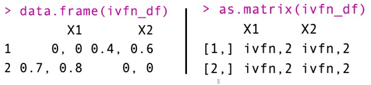
ivfn_df formats. The console output
for ivfn_fcm will vary depending on whether it is loaded as
a matrix or dataframe. If loaded as a dataframe it will print out IVFN
values. If loaded as a matrix it will print out object types (e.g.,
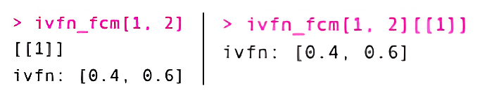
ivfn,2).To report the IVFN of a particular edge within an IVFN matrix, call
ivfn_fcm[row, col], which returns a list
object or ivfn_fcm[row, col][[1]] to return the first
record in the list object, the IVFN itself.
ivfn object organizationTo decompose an IVFN matrix into its upper and lower bounds, we can do the following:
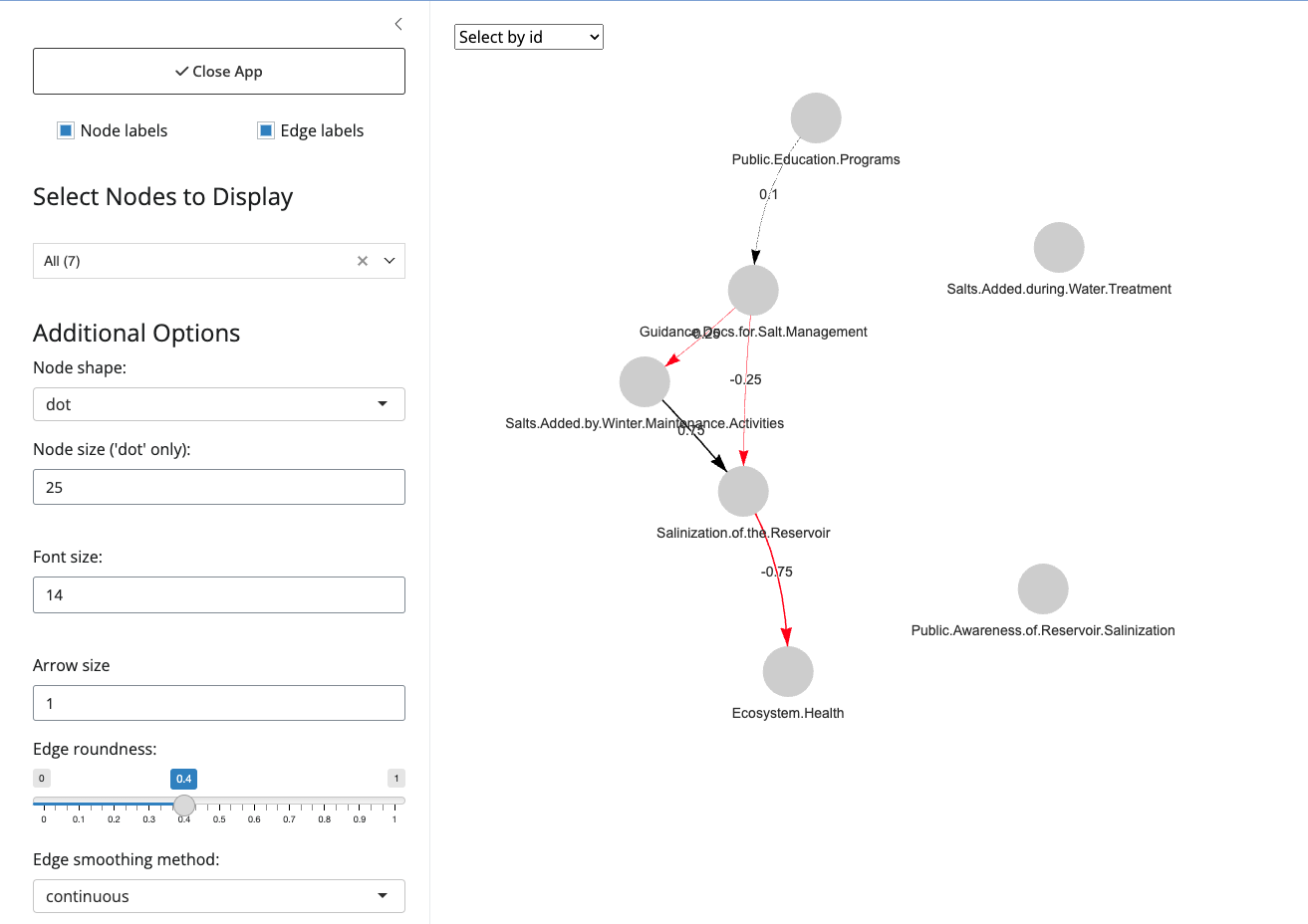
1.5 Viewing Imported FCMs
Users may display FCMs in RStudio’s Viewer pane using
fcm_view(), which plots an FCM (adjacency matrix) as a
visNetwork object. The resulting plot is interactive. Users
can manipulate node positions (i.e. the node layout) to explore the FCM
from different angles. The function can be used with any of the three
FCM types recognized by fcmconfr. For IVFN and TFN-FCMs,
fcm_view() plots the average edge weight to simplify the
node layout.
At its core, fcm_view() is just a call to
visNetwork functions. Users who have experience with
visNetwork should feel free to plot FCMs directly with
visNetwork for greater flexibility.
# Loading FCM from sample_fcms data
adj_matrix <- sample_fcms$simple_fcms$conventional_fcms[[1]]

# Show FCM in Viewer Pane
fcm_view(fcm_adj_matrix = adj_matrix)

# Store FCM visNetwork Object in a Variable
fcm_view_output <- fcm_view(fcm_adj_matrix = adj_matrix)
fcm_view_output # Shows FCM in Viewer Pane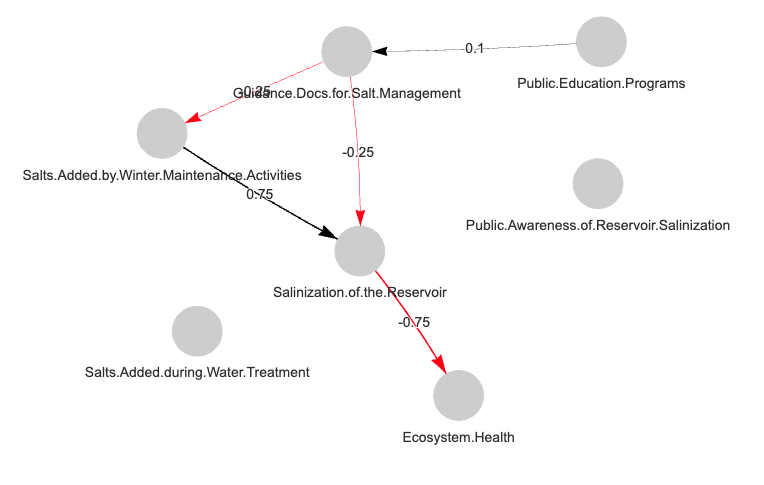
fcm_view() also offers more in-depth ways to interact
with FCM layouts through a GUI that can be accessed by adding
shiny = TRUE to the function call.
# Opens GUI but will not save output
fcm_view(fcm_adj_matrix = adj_matrix, shiny = TRUE)

# Opens GUI and will save output (into fcm_view_output)
fcm_view_output <- fcm_view(fcm_adj_matrix = adj_matrix, shiny = TRUE)
Note: By default, fcm_view() has an additional
parameter, alert_on_open , that users can set to
FALSE if they want to turn off the alert pop-up.
To open a saved output from fcm_view() in the GUI,
replace the fcm_adj_matrix parameter with
fcm_visNetwork. The following example shows how to reopen
the GUI with an fcm_view() output:
2. Set Simulation Parameters using fcmconfr_gui()
The primary fcmconfr() function is the central function
of the package and requires specifying many different parameters. The
fcmconfr_gui() function is intended to help guide users
through that process.
fcmconfr_gui() performs two tasks: (1) it launches a
Shiny app that lets users interactively select parameters and (2) it
outputs a corresponding call to fcmconfr() that users can
copy-and-paste to run in their own scripts.
No inputs are provided to fcmconfr_gui(), but the local
environment must have an individual FCM or a list object
containing multiple FCMs in order for fcmconfr_gui() to be
used. Once fcmconfr_gui() is running, select the
appropriate FCMs to analyze from a dropdown menu titled Adj. Matrix or
List of Adj. Matrices.
Matrices conforming to any of the above-noted FCM types (conventional, IVFN, or TFN) can be selected for analysis.

fcmconfr_gui() with
an example list of FCMs selected in the dropdown menu.The GUI interface is organized into four tabs: Data, Agg. and Monte Carlo Options, Simulation Options, and Runtime Options, which are described further below.
-
Data: The Data tab is where the user selects the FCMs they want to analyze (drop-down menu titled Adj. Matrix or List of Adj. Matrices). It is also where they manipulate values in the Initial State (Pulse) Vector or Clamping Vector to identify the dynamic simulations they wish to explore.
(Note: It is common to set every value in the Initial State (Pulse) Vector to 1 and to set only the node(s)-of-interest to 1 in the Clamping Vector. In this configuration, the Initial State (Pulse) Vector is used to determine the network’s state at equilibrium and the clamping vector is used to determine the network’s state in response to continuous activation of one or more nodes. The difference between the two is a measure of the impact of those particular nodes on the system.)
-
Agg. and Monte Carlo Options: The Agg. and Monte Carlo Options tab is where the user specifies their preferences regarding FCM aggregation and Monte Carlo sampling. Aggregation options are only available when datasets contain multiple FCMs. Monte Carlo sampling is available for
listobjects of conventional, IVFN- and TFN-FCMs as well as individual IVFN-/TFN-FCMs, but not individual conventional FCMs. Aggregation and Monte Carlo options can be toggled off to speed up the simulation process.Aggregation options allow the user to specify whether multiple FCMs should be aggregated into a single collective model so that dynamic simulations can be performed on the aggregate in addition to individual FCMs. The user can specify the aggregation method (mean or median) and whether zero-weighted edges should be included in the aggregation process. See
?aggregate_fcms()for more information on aggregating FCMs outside of the primaryfcmconfr()function.Monte Carlo options allow the user to specify whether Monte Carlo sampling should be performed to estimate uncertainty in dynamic simulation outputs. If yes, the user must specify the number of FCMs that will be generated by Monte Carlo sampling (we recommend 1000 or more). Dynamic simulations will be performed on each of these FCMs, providing a range of inferences for each node, from which the median state and quantiles (25th, 75th) will be estimated. The user also has the option to perform nonparametric bootstrapping to estimate confidence bounds about the average inference for each node. Confidence limits are user-specified (i.e., 95th percentile, 90th percentile, etc.).
Simulation Options: The Simulation Options tab is where users specify the type of dynamic simulation to perform. This includes specifying (1) the activation function (Kosko, Modified-Kosko, or Rescale; default of Kosko), (2) the squashing function (sigmoid or hyperbolic tangent; default of sigmoid), (3) the squashing function’s key parameter, lambda (default of 1), (4) the final simulation output (i.e., the peak estimate for each node or its final resting state; default of final), (5) the maximum number of iterations to perform per simulation (default of 100), and (6) the minimum acceptable error between iterations (default of 1x10⁻⁵)
Runtime Options: The Runtime Options tab allows the user to specify whether they want to use parallel processing and have a progress bar displayed at runtime. These options do not impact the simulation outputs. They do, however, influence how long
fcmconfr()takes to run and what the user sees at runtime.
A brief summary of each parameter within the
fcmconfr_gui() is provided in a glossary stored in a side
tab within the GUI. The side tab can be opened by clicking the arrow
symbol in the top-right-hand-corner of the GUI.
Once parameter selection is complete, click the ‘Get Code’ button at
the bottom of the GUI to display the corresponding code for a call to
fcmconfr() within the app.
The following code is an example output from
fcmconfr_gui().
fcmconfr(
  adj_matrices = sample_fcm_list,
  # Aggregation and Monte Carlo Sampling
  agg_function = 'mean',
  num_mc_fcms = 1000,
  # Simulation
  initial_state_vector = c(1, 1, 1, 1, 1, 1, 1),
  clamping_vector = c(1, 0, 0, 0, 0, 0, 0),
  activation = 'rescale',
  squashing = 'sigmoid',
  lambda = 1,
  point_of_inference = 'final',
  max_iter = 100,
  min_error = 1e-05,
  # Inference Estimation (bootstrap)
  ci_centering_function = 'mean',
  confidence_interval = 0.95,
  num_ci_bootstraps = 1000,
  # Runtime Options
  show_progress = TRUE,
  parallel = TRUE,
  n_cores = 2,
  # Additional Options
  run_agg_calcs = TRUE,
  run_mc_calcs = TRUE,
  run_ci_calcs = TRUE,
  include_zeroes_in_sampling = FALSE,
  include_sims_in_output = FALSE
)
Once the call to fcmconfr() has been generated by the
GUI, copy-and-paste it into another file and define it as a variable
(see example below):
fcmconfr_obj <- fcmconfr(
  adj_matrices = sample_fcm_list,
  # Aggregation and Monte Carlo Sampling
  agg_function = 'mean',
  num_mc_fcms = 1000,
  # Simulation
  initial_state_vector = c(1, 1, 1, 1, 1, 1, 1),
  clamping_vector = c(1, 0, 0, 0, 0, 0, 0),
  activation = 'rescale',
  squashing = 'sigmoid',
  lambda = 1,
  point_of_inference = 'final',
  max_iter = 100,
  min_error = 1e-05,
  # Inference Estimation (bootstrap)
  ci_centering_function = 'mean',
  confidence_interval = 0.95,
  num_ci_bootstraps = 1000,
  # Runtime Options
  show_progress = TRUE,
  parallel = TRUE,
  n_cores = 2,
  # Additional Options
  run_agg_calcs = TRUE,
  run_mc_calcs = TRUE,
  run_ci_calcs = TRUE,
  include_zeroes_in_sampling = FALSE,
  include_sims_in_output = FALSE
)
Click on ‘Close App’ or exit out of the shiny window to close the app.
Optional: Selecting an Appropriate Lambda
Lambda is set to 1 by default in fcmconfr. However,
there is no one “correct” value for lambda and values that work for one
FCM may not work for another. To give users a starting estimate for
lambda, fcmconfr provides the
estimate_lambda() function, which implements an algorithm
developed by Koutsellis et al. (2022) - https://doi.org/10.1007/s12351-022-00717-x.
estimate_lambda() returns the maximum lambda value that
guarantees simulation convergence (i.e. the max. usable value for
lambda) given a particular adjacency matrix and squashing function
(sigmoid or tanh).
An example call to estimate_lambda() has been provided
below.
example_fcm <- sample_fcms$simple_fcms$conventional_fcms[[1]]
estimate_lambda(example_fcm, squashing = "sigmoid")
estimate_lambda(example_fcm, squashing = "tanh")
The Koutsellis
et al. (2022) algorithm is intended for conventional FCMs. If an
IVFN-FCM or TFN-FCM is provided, estimate_lambda() will
create a conventional FCM by averaging the edge weights (upper and lower
for IVFN-FCMs and upper, mode, and lower for TFN-FCMs) for use in
calculating lambda.
example_ivfn_fcm <- sample_fcms$simple_fcms$ivfn_fcms[[1]]
example_tfn_fcm <- sample_fcms$simple_fcms$tfn_fcms[[1]]
estimate_lambda(example_ivfn_fcm, squashing = "sigmoid")
estimate_lambda(example_tfn_fcm, squashing = "sigmoid")
Since estimate_lambda() returns a different value for
each adjacency matrix, users will want to identify a value that will
work well with all FCMs being analyzed in each call to
fcmconfr(). Given this, we recommend estimating lambda
separately for each adjacency matrix and using the minimum lambda value
in fcmconfr(). See example below:
# Estimating lambda for dynamic simulations with multiple FCMs
example_fcms <- sample_fcms$simple_fcms$conventional_fcms

# Call lapply() to use estimate_lambda() on a list of FCMs.
lambda_estimates <- lapply(
  example_fcms, function(fcm) estimate_lambda(fcm, squashing = "sigmoid")
)

# Unlist the output lambda estimates to create a vector
# and calculate the minimum value
lambda_for_example_fcms <- min(unlist(lambda_estimates))

# Call fcmconfr using the estimated lambda value
fcmconfr_obj <- fcmconfr(
  adj_matrices = example_fcms,
  # Aggregation and Monte Carlo Sampling
  agg_function = 'mean',
  num_mc_fcms = 1000,
  # Simulation
  initial_state_vector = c(1, 1, 1, 1, 1, 1, 1),
  clamping_vector = c(1, 0, 0, 0, 0, 0, 0),
  activation = 'rescale',
  squashing = 'sigmoid',
  lambda = lambda_for_example_fcms, # Pass lambda estimate into fcmconfr() !!!!!
  point_of_inference = 'final',
  max_iter = 100,
  min_error = 1e-05,
  # Inference Estimation (bootstrap)
  ci_centering_function = 'mean',
  confidence_interval = 0.95,
  num_ci_bootstraps = 1000,
  # Runtime Options
  show_progress = TRUE,
  parallel = TRUE,
  n_cores = 2,
  # Additional Options
  run_agg_calcs = TRUE,
  run_mc_calcs = TRUE,
  run_ci_calcs = TRUE,
  include_zeroes_in_sampling = FALSE,
  include_sims_in_output = FALSE
)
Note: Because estimate_lambda() returns a potential
lambda value, not an optimal lambda value, users are encouraged to
compare the impact of different lambda choices on their simulation
results (e.g. lambda = 1, lambda = 0.1, lambda = 0.01, …).
3. Run fcmconfr()
To run fcmconfr(), execute the output script created by
fcmconfr_gui().
Note: When using parallel processing, the following error can occur:
Error in serialize(data, node$con) : error writing to connection.
If this error occurs, restart the R session and rerun
fcmconfr() with a lower value of n_cores.
4. Explore fcmconfr() Results
The output of fcmconfr() is a large object with many
compomnents. Given this, the fcmconfr package includes
several functions designed to help users identify and explore important
outputs.
The figure below graphically represents the organization of an
fcmconfr() object. Each branch represents a
list that can be accessed via
fcmconfr_obj$....
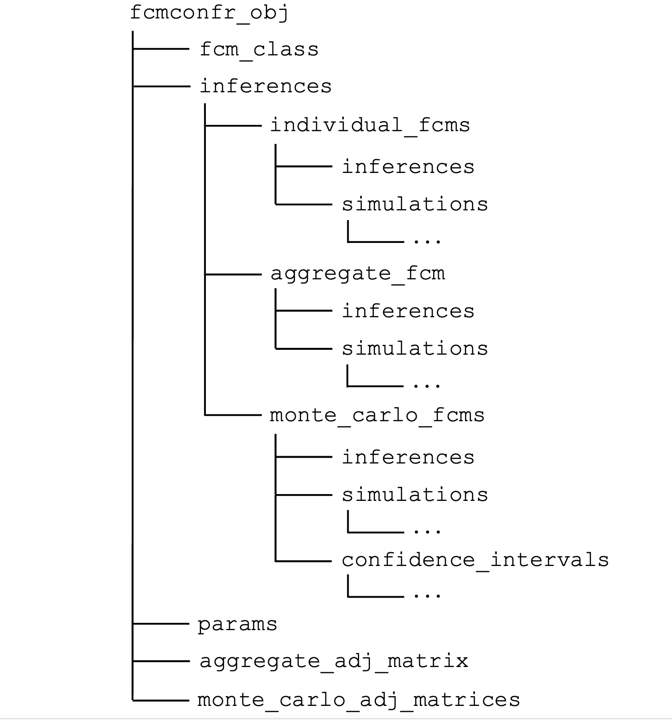
fcmconfr() output object. Three dots indicate additional
data within a branch.Note: The aggregate and Monte Carlo elements illustrated above
will only be included in fcmconfr() objects if
run_agg_calcs, run_mc_calcs,
run_ci_calcs, and include_sims_in_output are
set to TRUE respectively in the original
fcmconfr() call.
4.1 Visualizing fcmconfr() Results
A plot of all inferences included in the output of
fcmconfr() can be generated using the command
plot(fcmconfr_obj).
To view documentation for the version of plot() used by
fcmconfr output objects, type ?plot.fcmconfr
into the console. This provides definitions for all possible inputs
(i.e., beyond the fcmconfr object itself) that can be used
to customize the figure.
An example call illustrating the defaults for each input has been provided below:
# Plot Defaults
plot(fcmconfr_obj,
     interactive = FALSE, # Set to TRUE to open shiny app
     # Plot Formatting Parameters
     filter_limit = 1e-4,
     xlim = NA, # Axes limits - accepts c(lower_limit, upper_limit) inputs
     coord_flip = FALSE,
     # Plot Aesthetic Parameters
     mc_avg_and_CIs_color = "blue",
     mc_inferences_color = "blue",
     mc_inferences_alpha = 0.1, # scale from 0:transparent to 1:opaque
     mc_inferences_shape = 3, # R PCH point shape value (vertical cross)
     ind_inferences_color = "black",
     ind_inferences_alpha = 1, # scale from 0:transparent to 1:opaque
     ind_inferences_shape = 16, # R PCH point shape value (small circle)
     agg_inferences_color = "red",
     agg_inferences_alpha = 1, # scale from 0:transparent to 1:opaque
     agg_inferences_shape = 17, # R PCH point shape value (triangle)
     ind_ivfn_and_tfn_linewidth = 0.1,
     agg_ivfn_and_tfn_linewidth = 0.6
)
The interactive parameter in the call to
plot() allows users to launch the plot inside a Shiny app
where the results from different analyses can be toggled on/off
(interactive = TRUE). This is a great option for data
exploration. Note: It may be necessary to experiment with
font size within the app to clearly view axis labels.
An example call, where the interactive parameter is set
to TRUE and the x-axis is constrained between -0.5 and 0.5
has been provided below:
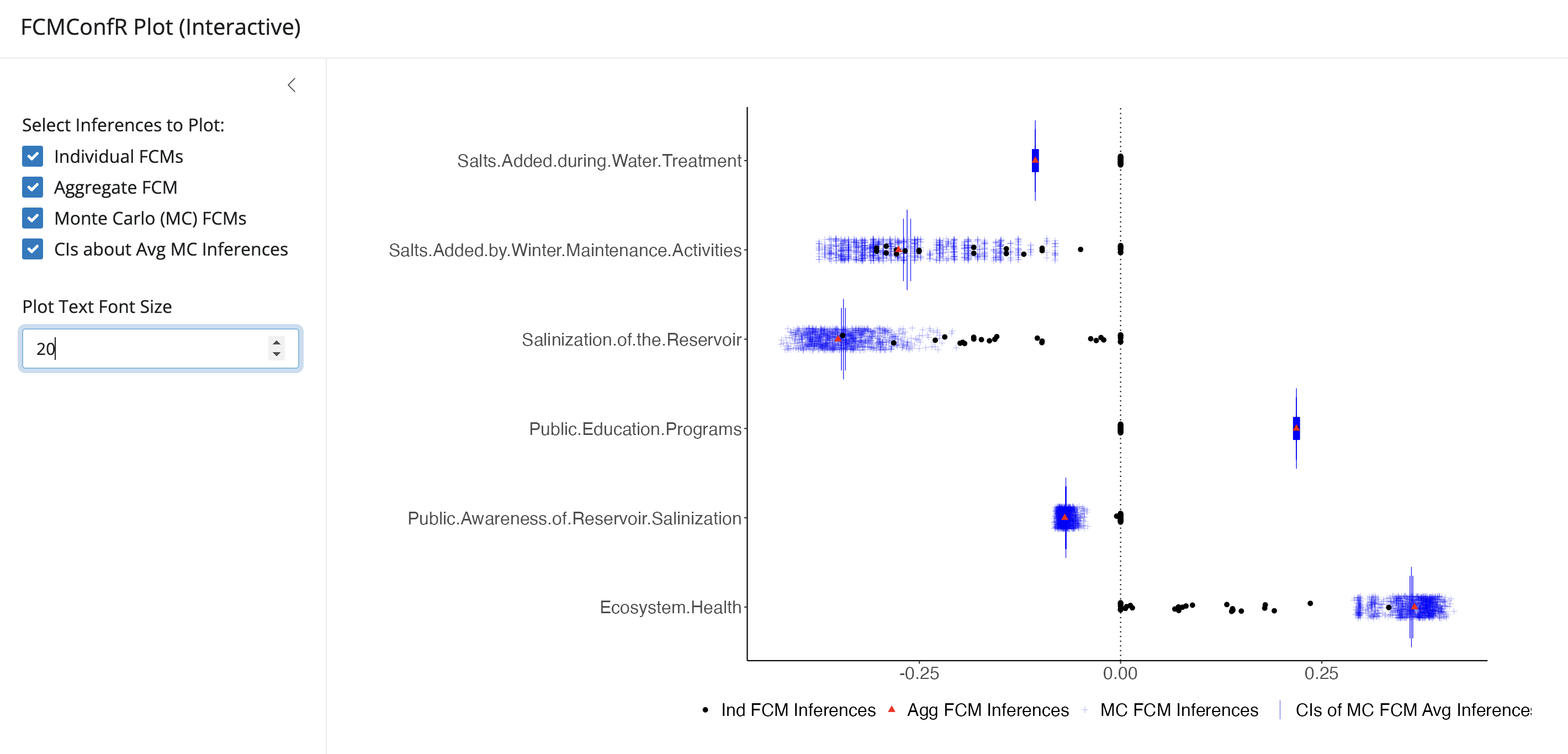
fcmconfr() object launched inside the Shiny app (user
controls on left; plot on right).4.2 Retrieving Inferences with get_fcmconfr_inferences()
Simulation inferences (individual, aggregate, Monte Carlo) are the
main output from fcmconfr(). They indicate how much each
node is influenced by a particular change or action. Inferences can be
accessed as follows:
all_inferences <- fcmconfr_obj$inferences

individual_fcm_inferences <- all_inferences$individual_fcms$inferences
aggregate_fcm_inferences <- all_inferences$aggregate_fcm$inferences
mc_fcm_inferences <- all_inferences$monte_carlo_fcms$all_inferences
CIs_of_avg_mc_fcm_inferences <- all_inferences$monte_carlo_fcms$bootstrap$CIs_and_quantiles_by_node
In addition to accessing inference data manually (as shown above),
fcmconfr provides the
get_fcmconfr_inferences() function to retrieve and store
inference results.
fcmconfr_inferences <- get_fcmconfr_inferences(fcmconfr_obj, analysis = c("individual", "aggregate", "mc"))The output of get_fcmconfr_inferences() is a
list of dataframes containing the inferences for each
analysis. By default,
analysis = c("individual", "aggregate", "mc"), but users
can also specify a subset of these categories.
When "mc" is included and the box for bootstrapped
confidence intervals is checked, get_fcmconfr_inferences()
returns two types of MC outputs: (1) inferences from each empirical FCM
generated by Monte Carlo sampling and (2) a dataframe containing user
specified bootstrapped confidence bounds about the average of those
inferences.
4.3 Retrieving Inferences with summary()
Users can also access a simplified output of fcmconfr()
inferences using the summary() function on an
fcmconfr() output object.
summary(fcmconfr_obj)summary() also prints information about the inferences
across each analysis performed to create the fcmconfr()
output. An example of a summary(fcmconfr_obj) output for an
analysis of IVFN-FCMs that only calculated inferences for the individual
and aggregate adjacency matrices is given below:
~~~~~ Summary ~~~~~

$individual_inferences
                                                             Median                   Mean
Guidance.Docs.for.Salt.Management                           1, 1, 1                1, 1, 1
Public.Education.Programs                                   0, 0, 0    0.002, 0.007, 0.011
Salts.Added.during.Water.Treatment                          0, 0, 0                0, 0, 0
Salts.Added.by.Winter.Maintenance.Activities  -0.250, -0.097, 0.000 -0.175, -0.118, -0.043
Ecosystem.Health                                0.012, 0.064, 0.088    0.034, 0.071, 0.092
Public.Awareness.of.Reservoir.Salinization                  0, 0, 0   -0.001, 0.000, 0.000
Salinization.of.the.Reservoir                -0.139, -0.092, -0.012 -0.144, -0.100, -0.038

$aggregate_inferences
                                              crisp  lower   mode  upper
Guidance.Docs.for.Salt.Management             1.000  1.000  1.000  1.000
Public.Education.Programs                     0.008  0.002  0.008  0.015
Salts.Added.during.Water.Treatment            0.000  0.000  0.000  0.000
Salts.Added.by.Winter.Maintenance.Activities -0.131 -0.212 -0.136 -0.046
Ecosystem.Health                              0.076  0.034  0.080  0.115
Public.Awareness.of.Reservoir.Salinization   -0.001 -0.002 -0.001  0.000
Salinization.of.the.Reservoir                -0.119 -0.187 -0.124 -0.045

┌────────────────────────────────────────────────────────────────┐
│                                                                │
│   Inferences via fcmconfr: 30 individual adj. matrices (tfn)   │
│                                                                │
└────────────────────────────────────────────────────────────────┘
Advanced Inference Options
FCM inferences are calculated from FCM simulations, which can include hundreds of iterations for each node in each FCM (individual, aggregate, and Monte Carlo).
The get_fcmconfr_inferences() function returns standard
inference estimates only (e.g., the final point of convergence for each
node or the peak simulated value for each node, as specified in the
original call to fcmconfr())
Users interested in calculating their own inferences directly from simulation time-series can access that data as follows:
# Simulations for individual_fcms
individual_fcms_sims <- fcmconfr_obj$inferences$individual_fcms$simulations

# Simulations for aggregate_fcm
aggregate_fcm_sims <- fcmconfr_obj$inferences$aggregate_fcm$simulations

# Simulations for monte_carlo_fcms
monte_carlo_fcms_sims <- fcmconfr_obj$inferences$monte_carlo_fcms$simulations
These commands return a list of the simulations for
every adjacency matrix in a given analysis. Users can retrieve
simulations for a specific adjacency matrix (e.g.,
adj_matrix_1 from individual_fcms_sims) as
follows:
sim_1 <- individual_fcms_sims$adj_matrix_1$simulationsThis returns both the scenario_simulation and
baseline_simulation data for a given adjacency matrix.
The scenario_simulation outputs incorporate the clamping
vector, so we observe the influence of continuously activating
(“clamping”) one (or some) nodes.
The baseline_simulation outputs incorporate ONLY the
initial state vector, so we observe the steady-state (or natural
behavior) of the system as a control.
Inferences are calculated by taking the difference between the two
(scenario - baseline). Different metrics are used for
peak vs final inferences as described
below:
# Continuing from the example above
# Get the state vectors for the scenario simulation
scenario_state_vectors <- sim_1$scenario_simulation$state_vectors
# Get the state vectors for the baseline simulation
baseline_state_vectors <- sim_1$baseline_simulation$state_vectors
# Calculating final inferences
# Same as fcmconfr() output with point_of_inference = 'final'
scenario_sim_final_values <- scenario_state_vectors[nrow(scenario_state_vectors), ]
baseline_sim_final_values <- baseline_state_vectors[nrow(baseline_state_vectors), ]
individual_fcm_1_final_inferences <- scenario_sim_final_values - baseline_sim_final_values
# Calculating peak inferences
# Same as fcmconfr() output with point_of_inference = 'peak'
# Note: Peak will not work unless all values in the clamping vector are 0!
scenario_sim_peak_values <- t(apply(
scenario_state_vectors, 2, function(col) {unique(col[abs(col) == max(abs(col))])}
))
baseline_sim_peak_values <- t(apply(
baseline_state_vectors, 2, function(col) {unique(col[abs(col) == max(abs(col))])}
))
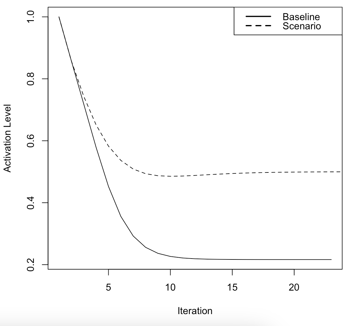
individual_fcm_1_peak_inferences <- scenario_sim_peak_values - baseline_sim_peak_valuesUsers can view scenario and baseline
simulation time-series for specific nodes (e.g.,
Salinization.of.the.Reservoir) as described below. The
difference between the scenario and baseline
time-series is the inference.
salinization_scenario_time_series <- scenario_state_vectors$Salinization.of.the.Reservoir
salinization_baseline_time_series <- baseline_state_vectors$Salinization.of.the.Reservoir

plot(salinization_scenario_time_series, type = "l",
      xlab = "Iteration", ylab = "Activation Level")
lines(salinization_baseline_time_series, lty = "dashed")
legend(x = "topright",
       legend = c("Baseline", "Scenario"),
       lty = c(1, 2),
       lwd = 2)